Sine and cosine
Fundamental trigonometric functions
| Sine and cosine | |
|---|---|
 | |
| General information | |
| General definition | |
| Fields of application | Trigonometry, Fourier series, etc. |
![{\displaystyle {\begin{aligned}&\sin(\alpha )={\frac {\textrm {opposite}}{\textrm {hypotenuse}}}\\[8pt]&\cos(\alpha )={\frac {\textrm {adjacent}}{\textrm {hypotenuse}}}\\[8pt]\end{aligned}}}](https://wikimedia.org/api/rest_v1/media/math/render/svg/ea2762f231f5fdc1dcfacd59c303106f596ab2e1)
| Trigonometry |
|---|
 |
|
| Reference |
|
| Laws and theorems |
|
| Calculus |
| Mathematicians |
|
In mathematics, sine and cosine are trigonometric functions of an angle. The sine and cosine of an acute angle are defined in the context of a right triangle: for the specified angle, its sine is the ratio of the length of the side that is opposite that angle to the length of the longest side of the triangle (the hypotenuse), and the cosine is the ratio of the length of the adjacent leg to that of the hypotenuse. For an angle , the sine and cosine functions are denoted as and .


The definitions of sine and cosine have been extended to any real value in terms of the lengths of certain line segments in a unit circle. More modern definitions express the sine and cosine as infinite series, or as the solutions of certain differential equations, allowing their extension to arbitrary positive and negative values and even to complex numbers.
The sine and cosine functions are commonly used to model periodic phenomena such as sound and light waves, the position and velocity of harmonic oscillators, sunlight intensity and day length, and average temperature variations throughout the year. They can be traced to the jyā and koṭi-jyā functions used in Indian astronomy during the Gupta period.
Elementary descriptions
Right-angled triangle definition

To define the sine and cosine of an acute angle , start with a right triangle that contains an angle of measure ; in the accompanying figure, angle in a right triangle is the angle of interest. The three sides of the triangle are named as follows:[1]


- The opposite side is the side opposite to the angle of interest; in this case, it is .
- The hypotenuse is the side opposite the right angle; in this case, it is . The hypotenuse is always the longest side of a right-angled triangle.
- The adjacent side is the remaining side; in this case, it is . It forms a side of (and is adjacent to) both the angle of interest and the right angle.


Once such a triangle is chosen, the sine of the angle is equal to the length of the opposite side divided by the length of the hypotenuse, and the cosine of the angle is equal to the length of the adjacent side divided by the length of the hypotenuse:[1]

Other trigonometric functions
The other trigonometric functions of the angle can be defined similarly; for example, the tangent is the ratio between the opposite and adjacent sides or equivalently the ratio between the sine and cosine functions. The reciprocal of sine is cosecant, which gives the ratio of the hypotenuse length to the length of the opposite side. Similarly, the reciprocal of cosine is secant, which gives the ratio of the hypotenuse length to that of the adjacent side. The cotangent function is the ratio between the adjacent and opposite sides, a reciprocal of a tangent function. These functions can be formulated as:[1]

Special angle measures
As stated, the values and appear to depend on the choice of a right triangle containing an angle of measure . However, this is not the case as all such triangles are similar, and so the ratios are the same for each of them. For example, each leg of the 45-45-90 right triangle is 1 unit, and its hypotenuse is ; therefore, .[2] The following table shows the special value of each input for both sine and cosine with the domain between . The input in this table provides various unit systems such as degree, radian, and so on. The angles other than those five can be obtained by using a calculator.[3][4]


| Angle, x | sin(x) | cos(x) | |||||
|---|---|---|---|---|---|---|---|
| Degrees | Radians | Gradians | Turns | Exact | Decimal | Exact | Decimal |
| 0° | 0 | 0g | 0 | 0 | 0 | 1 | 1 |
| 30° | 1/6π | 33+1/3g | 1/12 | 1/2 | 0.5 | 0.8660 | |
| 45° | 1/4π | 50g | 1/8 | 0.7071 | 0.7071 | ||
| 60° | 1/3π | 66+2/3g | 1/6 | 0.8660 | 1/2 | 0.5 | |
| 90° | 1/2π | 100g | 1/4 | 1 | 1 | 0 | 0 |


Laws

The law of sines is useful for computing the lengths of the unknown sides in a triangle if two angles and one side are known.[5] Given that a triangle with sides , , and , and angles opposite those sides , , and . The law states, This is equivalent to the equality of the first three expressions below: where is the triangle's circumradius.


The law of cosines is useful for computing the length of an unknown side if two other sides and an angle are known.[5] The law states, In the case where from which , the resulting equation becomes the Pythagorean theorem.[6]


Vector definition
The cross product and dot product are operations on two vectors in Euclidean vector space. The sine and cosine functions can be defined in terms of the cross product and dot product. If and are vectors, and is the angle between and , then sine and cosine can be defined as:


Analytic descriptions
Unit circle definition
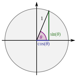
The sine and cosine functions may also be defined in a more general way by using unit circle, a circle of radius one centered at the origin , formulated as the equation of in the Cartesian coordinate system. Let a line through the origin intersect the unit circle, making an angle of with the positive half of the -axis. The - and -coordinates of this point of intersection are equal to and , respectively; that is,[7]


This definition is consistent with the right-angled triangle definition of sine and cosine when because the length of the hypotenuse of the unit circle is always 1; mathematically speaking, the sine of an angle equals the opposite side of the triangle, which is simply the -coordinate. A similar argument can be made for the cosine function to show that the cosine of an angle when , even under the new definition using the unit circle.[8][9]

Graph of a function and its elementary properties

Using the unit circle definition has the advantage of drawing a graph of sine and cosine functions. This can be done by rotating counterclockwise a point along the circumference of a circle, depending on the input . In a sine function, if the input is , the point is rotated counterclockwise and stopped exactly on the -axis. If , the point is at the circle's halfway. If , the point returned to its origin. This results that both sine and cosine functions have the range between .[10]


Extending the angle to any real domain, the point rotated counterclockwise continuously. This can be done similarly for the cosine function as well, although the point is rotated initially from the -coordinate. In other words, both sine and cosine functions are periodic, meaning any angle added by the circumference's circle is the angle itself. Mathematically,[11]

A function is said to be odd if , and is said to be even if . The sine function is odd, whereas the cosine function is even.[12] Both sine and cosine functions are similar, with their difference being shifted by . This means,[13]


Zero is the only real fixed point of the sine function; in other words the only intersection of the sine function and the identity function is . The only real fixed point of the cosine function is called the Dottie number. The Dottie number is the unique real root of the equation . The decimal expansion of the Dottie number is approximately 0.739085.[14]


Continuity and differentiation

The sine and cosine functions are infinitely differentiable.[15] The derivative of sine is cosine, and the derivative of cosine is negative sine:[16] Continuing the process in higher-order derivative results in the repeated same functions; the fourth derivative of a sine is the sine itself.[15] These derivatives can be applied to the first derivative test, according to which the monotonicity of a function can be defined as the inequality of function's first derivative greater or less than equal to zero.[17] It can also be applied to second derivative test, according to which the concavity of a function can be defined by applying the inequality of the function's second derivative greater or less than equal to zero.[18] The following table shows that both sine and cosine functions have concavity and monotonicity—the positive sign () denotes a graph is increasing (going upward) and the negative sign () is decreasing (going downward)—in certain intervals.[19] This information can be represented as a Cartesian coordinates system divided into four quadrants.


| Quadrant | Angle | Sine | Cosine | |||||
|---|---|---|---|---|---|---|---|---|
| Degrees | Radians | Sign | Monotony | Convexity | Sign | Monotony | Convexity | |
| 1st quadrant, I | increasing | concave | decreasing | concave | ||||
| 2nd quadrant, II | decreasing | concave | decreasing | convex | ||||
| 3rd quadrant, III | decreasing | convex | increasing | convex | ||||
| 4th quadrant, IV | increasing | convex | increasing | concave | ||||


Both sine and cosine functions can be defined by using differential equations. The pair of is the solution to the two-dimensional system of differential equations and with the initial conditions and . One could interpret the unit circle in the above definitions as defining the phase space trajectory of the differential equation with the given initial conditions. It can be interpreted as a phase space trajectory of the system of differential equations and starting from the initial conditions and .[citation needed]


Integral and the usage in mensuration
Their area under a curve can be obtained by using the integral with a certain bounded interval. Their antiderivatives are: where denotes the constant of integration.[20] These antiderivatives may be applied to compute the mensuration properties of both sine and cosine functions' curves with a given interval. For example, the arc length of the sine curve between and is where is the incomplete elliptic integral of the second kind with modulus . It cannot be expressed using elementary functions.[21] In the case of a full period, its arc length is where is the gamma function and is the lemniscate constant.[22]


Inverse functions

The inverse function of sine is arcsine or inverse sine, denoted as "arcsin", "asin", or .[23] The inverse function of cosine is arccosine, denoted as "arccos", "acos", or .[a] As sine and cosine are not injective, their inverses are not exact inverse functions, but partial inverse functions. For example, , but also , , and so on. It follows that the arcsine function is multivalued: , but also , , and so on. When only one value is desired, the function may be restricted to its principal branch. With this restriction, for each in the domain, the expression will evaluate only to a single value, called its principal value. The standard range of principal values for arcsin is from to , and the standard range for arccos is from to .[24]


The inverse function of both sine and cosine are defined as:[citation needed] where for some integer , By definition, both functions satisfy the equations:[citation needed] and


Other identities
According to Pythagorean theorem, the squared hypotenuse is the sum of two squared legs of a right triangle. Dividing the formula on both sides with squared hypotenuse resulting in the Pythagorean trigonometric identity, the sum of a squared sine and a squared cosine equals 1:[25][b]

Sine and cosine satisfy the following double-angle formulas:[citation needed]


The cosine double angle formula implies that sin2 and cos2 are, themselves, shifted and scaled sine waves. Specifically,[26] The graph shows both sine and sine squared functions, with the sine in blue and the sine squared in red. Both graphs have the same shape but with different ranges of values and different periods. Sine squared has only positive values, but twice the number of periods.[citation needed]

Series and polynomials

Both sine and cosine functions can be defined by using a Taylor series, a power series involving the higher-order derivatives. As mentioned in § Continuity and differentiation, the derivative of sine is cosine and that the derivative of cosine is the negative of sine. This means the successive derivatives of are , , , , continuing to repeat those four functions. The -th derivative, evaluated at the point 0: where the superscript represents repeated differentiation. This implies the following Taylor series expansion at . One can then use the theory of Taylor series to show that the following identities hold for all real numbers —where is the angle in radians.[27] More generally, for all complex numbers:[28] Taking the derivative of each term gives the Taylor series for cosine:[27][28]


Both sine and cosine functions with multiple angles may appear as their linear combination, resulting in a polynomial. Such a polynomial is known as the trigonometric polynomial. The trigonometric polynomial's ample applications may be acquired in its interpolation, and its extension of a periodic function known as the Fourier series. Let and be any coefficients, then the trigonometric polynomial of a degree —denoted as —is defined as:[29][30]


The trigonometric series can be defined similarly analogous to the trigonometric polynomial, its infinite inversion. Let and be any coefficients, then the trigonometric series can be defined as:[31] In the case of a Fourier series with a given integrable function , the coefficients of a trigonometric series are:[32]


Complex numbers relationship
Complex exponential function definitions
Both sine and cosine can be extended further via complex number, a set of numbers composed of both real and imaginary numbers. For real number , the definition of both sine and cosine functions can be extended in a complex plane in terms of an exponential function as follows:[33]

Alternatively, both functions can be defined in terms of Euler's formula:[33]

When plotted on the complex plane, the function for real values of traces out the unit circle in the complex plane. Both sine and cosine functions may be simplified to the imaginary and real parts of as:[34]


When for real values and , where , both sine and cosine functions can be expressed in terms of real sines, cosines, and hyperbolic functions as:[citation needed]


Polar coordinates

Sine and cosine are used to connect the real and imaginary parts of a complex number with its polar coordinates : and the real and imaginary parts are: where and represents the magnitude and angle of the complex number .


For any real number , Euler's formula in terms of polar coordinates is stated as .

Complex arguments


Applying the series definition of the sine and cosine to a complex argument, z, gives:

where sinh and cosh are the hyperbolic sine and cosine. These are entire functions.
It is also sometimes useful to express the complex sine and cosine functions in terms of the real and imaginary parts of its argument:

Partial fraction and product expansions of complex sine
Using the partial fraction expansion technique in complex analysis, one can find that the infinite series both converge and are equal to . Similarly, one can show that


Using product expansion technique, one can derive Alternatively, the infinite product for the sine can be proved using complex Fourier series.[c]

Usage of complex sine
sin(z) is found in the functional equation for the Gamma function,

which in turn is found in the functional equation for the Riemann zeta-function,

As a holomorphic function, sin z is a 2D solution of Laplace's equation:

The complex sine function is also related to the level curves of pendulums.[how?][36][better source needed]
Complex graphs
 | 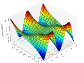 |  |
| real component | imaginary component | magnitude |
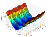
 | 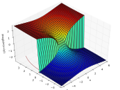 |  |
| real component | imaginary component | magnitude |
Background
Etymology
The word sine is derived, indirectly, from the Sanskrit word jyā 'bow-string' or more specifically its synonym jīvá (both adopted from Ancient Greek χορδή 'string', due to visual similarity between the arc of a circle with its corresponding chord and a bow with its string (see jyā, koti-jyā and utkrama-jyā). This was transliterated in Arabic as jība, which is meaningless in that language and written as jb (جب). Since Arabic is written without short vowels, jb was interpreted as the homograph jayb (جيب), which means 'bosom', 'pocket', or 'fold'.[37][38] When the Arabic texts of Al-Battani and al-Khwārizmī were translated into Medieval Latin in the 12th century by Gerard of Cremona, he used the Latin equivalent sinus (which also means 'bay' or 'fold', and more specifically 'the hanging fold of a toga over the breast').[39][40][41] Gerard was probably not the first scholar to use this translation; Robert of Chester appears to have preceded him and there is evidence of even earlier usage.[42][43] The English form sine was introduced in the 1590s.[d]
The word cosine derives from an abbreviation of the Latin complementi sinus 'sine of the complementary angle' as cosinus in Edmund Gunter's Canon triangulorum (1620), which also includes a similar definition of cotangens.[44]
History

While the early study of trigonometry can be traced to antiquity, the trigonometric functions as they are in use today were developed in the medieval period. The chord function was discovered by Hipparchus of Nicaea (180–125 BCE) and Ptolemy of Roman Egypt (90–165 CE).[45]
The sine and cosine functions can be traced to the jyā and koṭi-jyā functions used in Indian astronomy during the Gupta period (Aryabhatiya and Surya Siddhanta), via translation from Sanskrit to Arabic and then from Arabic to Latin.[39]
All six trigonometric functions in current use were known in Islamic mathematics by the 9th century, as was the law of sines, used in solving triangles.[46] With the exception of the sine (which was adopted from Indian mathematics), the other five modern trigonometric functions were discovered by Arabic mathematicians, including the cosine, tangent, cotangent, secant and cosecant.[46] Al-Khwārizmī (c. 780–850) produced tables of sines, cosines and tangents.[47][48] Muhammad ibn Jābir al-Harrānī al-Battānī (853–929) discovered the reciprocal functions of secant and cosecant, and produced the first table of cosecants for each degree from 1° to 90°.[48]
The first published use of the abbreviations sin, cos, and tan is by the 16th-century French mathematician Albert Girard; these were further promulgated by Euler (see below). The Opus palatinum de triangulis of Georg Joachim Rheticus, a student of Copernicus, was probably the first in Europe to define trigonometric functions directly in terms of right triangles instead of circles, with tables for all six trigonometric functions; this work was finished by Rheticus' student Valentin Otho in 1596.
In a paper published in 1682, Leibniz proved that sin x is not an algebraic function of x.[49] Roger Cotes computed the derivative of sine in his Harmonia Mensurarum (1722).[50] Leonhard Euler's Introductio in analysin infinitorum (1748) was mostly responsible for establishing the analytic treatment of trigonometric functions in Europe, also defining them as infinite series and presenting "Euler's formula", as well as the near-modern abbreviations sin., cos., tang., cot., sec., and cosec.[39]
Software implementations
There is no standard algorithm for calculating sine and cosine. IEEE 754, the most widely used standard for the specification of reliable floating-point computation, does not address calculating trigonometric functions such as sine. The reason is that no efficient algorithm is known for computing sine and cosine with a specified accuracy, especially for large inputs.[51]
Algorithms for calculating sine may be balanced for such constraints as speed, accuracy, portability, or range of input values accepted. This can lead to different results for different algorithms, especially for special circumstances such as very large inputs, e.g. sin(1022).
A common programming optimization, used especially in 3D graphics, is to pre-calculate a table of sine values, for example one value per degree, then for values in-between pick the closest pre-calculated value, or linearly interpolate between the 2 closest values to approximate it. This allows results to be looked up from a table rather than being calculated in real time. With modern CPU architectures this method may offer no advantage.[citation needed]
The CORDIC algorithm is commonly used in scientific calculators.
The sine and cosine functions, along with other trigonometric functions, are widely available across programming languages and platforms. In computing, they are typically abbreviated to sin and cos.
Some CPU architectures have a built-in instruction for sine, including the Intel x87 FPUs since the 80387.
In programming languages, sin and cos are typically either a built-in function or found within the language's standard math library. For example, the C standard library defines sine functions within math.h: sin(double), sinf(float), and sinl(long double). The parameter of each is a floating point value, specifying the angle in radians. Each function returns the same data type as it accepts. Many other trigonometric functions are also defined in math.h, such as for cosine, arc sine, and hyperbolic sine (sinh). Similarly, Python defines math.sin(x) and math.cos(x) within the built-in math module. Complex sine and cosine functions are also available within the cmath module, e.g. cmath.sin(z). CPython's math functions call the C math library, and use a double-precision floating-point format.
Turns based implementations
Some software libraries provide implementations of sine and cosine using the input angle in half-turns, a half-turn being an angle of 180 degrees or radians. Representing angles in turns or half-turns has accuracy advantages and efficiency advantages in some cases.[52][53] In MATLAB, OpenCL, R, Julia, CUDA, and ARM, these functions are called sinpi and cospi.[52][54][53][55][56][57] For example, sinpi(x) would evaluate to where x is expressed in half-turns, and consequently the final input to the function, πx can be interpreted in radians by sin.

The accuracy advantage stems from the ability to perfectly represent key angles like full-turn, half-turn, and quarter-turn losslessly in binary floating-point or fixed-point. In contrast, representing , , and in binary floating-point or binary scaled fixed-point always involves a loss of accuracy since irrational numbers cannot be represented with finitely many binary digits.

Turns also have an accuracy advantage and efficiency advantage for computing modulo to one period. Computing modulo 1 turn or modulo 2 half-turns can be losslessly and efficiently computed in both floating-point and fixed-point. For example, computing modulo 1 or modulo 2 for a binary point scaled fixed-point value requires only a bit shift or bitwise AND operation. In contrast, computing modulo involves inaccuracies in representing .
For applications involving angle sensors, the sensor typically provides angle measurements in a form directly compatible with turns or half-turns. For example, an angle sensor may count from 0 to 4096 over one complete revolution.[58] If half-turns are used as the unit for angle, then the value provided by the sensor directly and losslessly maps to a fixed-point data type with 11 bits to the right of the binary point. In contrast, if radians are used as the unit for storing the angle, then the inaccuracies and cost of multiplying the raw sensor integer by an approximation to would be incurred.

See also
- Āryabhaṭa's sine table
- Bhaskara I's sine approximation formula
- Discrete sine transform
- Dixon elliptic functions
- Euler's formula
- Generalized trigonometry
- Hyperbolic function
- Lemniscate elliptic functions
- Law of sines
- List of periodic functions
- List of trigonometric identities
- Madhava series
- Madhava's sine table
- Optical sine theorem
- Polar sine—a generalization to vertex angles
- Proofs of trigonometric identities
- Sinc function
- Sine and cosine transforms
- Sine integral
- Sine quadrant
- Sine wave
- Sine–Gordon equation
- Sinusoidal model
- SOH-CAH-TOA
- Trigonometric functions
- Trigonometric integral
References
Footnotes
- ^ The superscript of −1 in and denotes the inverse of a function, instead of exponentiation.
- ^ Here, means the squared sine function .
- ^ Using complex Fourier series, the function can be decomposed as Setting yields Therefore, The function is the derivative of . Furthermore, if , then the function such that the emerged series converges on some open and connected subset of is , which can be proved using the Weierstrass M-test. The interchange of the sum and derivative is justified by uniform convergence. It follows that Exponentiating gives Since and , it results in . Hence, for some open and connected subset of . Let . Since converges uniformly on any closed disk, converges uniformly on any closed disk as well.[35] It follows that the infinite product is holomorphic on . By the identity theorem, the infinite product for the sine is valid for all , which completes the proof.
- ^ The anglicized form is first recorded in 1593 in Thomas Fale's Horologiographia, the Art of Dialling.


![{\displaystyle \cos(zx)={\frac {z\sin(\pi z)}{\pi }}\displaystyle \sum _{n=-\infty }^{\infty }{\frac {(-1)^{n}\,e^{inx}}{z^{2}-n^{2}}},\,z\in \mathbb {C} \setminus \mathbb {Z} ,\,x\in [-\pi ,\pi ].}](https://wikimedia.org/api/rest_v1/media/math/render/svg/4344e0e79e6b3e4af5cabc1ae8ac71054f88e915)


Citations
- ^ a b c Young (2017), p. 27.
- ^ Young (2017), p. 36.
- ^ Varberg, Purcell & Rigdon (2007), p. 42.
- ^ Young (2017), p. 37, 78.
- ^ a b Axler (2012), p. 634.
- ^ Axler (2012), p. 632.
- ^ Varberg, Purcell & Rigdon (2007), p. 41.
- ^ Young (2017), p. 68.
- ^ Varberg, Purcell & Rigdon (2007), p. 47.
- ^ Varberg, Purcell & Rigdon (2007), p. 41–42.
- ^ Varberg, Purcell & Rigdon (2007), p. 41, 43.
- ^ Young (2012), p. 165.
- ^ Varberg, Purcell & Rigdon (2007), p. 42, 47.
- ^ "OEIS A003957". oeis.org. Retrieved 2019-05-26.
- ^ a b Bourchtein & Bourchtein (2022), p. 294.
- ^ Varberg, Purcell & Rigdon (2007), p. 115.
- ^ Varberg, Purcell & Rigdon (2007), p. 155.
- ^ Varberg, Purcell & Rigdon (2007), p. 157.
- ^ Varberg, Rigdon & Purcell (2007), p. 42. sfnp error: no target: CITEREFVarbergRigdonPurcell2007 (help)
- ^ Varberg, Purcell & Rigdon (2007), p. 199.
- ^ Vince (2023), p. 162.
- ^ Adlaj (2012).
- ^ Varberg, Purcell & Rigdon (2007), p. 366.
- ^ Varberg, Purcell & Rigdon (2007), p. 365.
- ^ Young (2017), p. 99.
- ^ "Sine-squared function". Retrieved August 9, 2019.
- ^ a b Varberg, Purcell & Rigdon (2007), p. 491–492.
- ^ a b Abramowitz & Stegun (1970), p. 74.
- ^ Powell (1981), p. 150.
- ^ Rudin (1987), p. 88.
- ^ Zygmund (1968), p. 1.
- ^ Zygmund (1968), p. 11.
- ^ a b Howie (2003), p. 24.
- ^ Rudin (1987), p. 2.
- ^ Rudin (1987), p. 299, Theorem 15.4.
- ^ "Why are the phase portrait of the simple plane pendulum and a domain coloring of sin(z) so similar?". math.stackexchange.com. Retrieved 2019-08-12.
- ^ Plofker (2009), p. 257.
- ^ Maor (1998), p. 35.
- ^ a b c Merzbach & Boyer (2011).
- ^ Maor (1998), p. 35–36.
- ^ Katz (2008), p. 253.
- ^ Smith (1958), p. 202.
- ^ Various sources credit the first use of sinus to either
- Plato Tiburtinus's 1116 translation of the Astronomy of Al-Battani
- Gerard of Cremona's translation of the Algebra of al-Khwārizmī
- Robert of Chester's 1145 translation of the tables of al-Khwārizmī
- ^ Gunter (1620).
- ^ Brendan, T. (February 1965). "How Ptolemy constructed trigonometry tables". The Mathematics Teacher. 58 (2): 141–149. doi:10.5951/MT.58.2.0141. JSTOR 27967990 – via JSTOR.
- ^ a b Gingerich, Owen (1986). "Islamic Astronomy". Scientific American. Vol. 254. p. 74. Archived from the original on 2013-10-19. Retrieved 2010-07-13.
- ^ Jacques Sesiano, "Islamic mathematics", p. 157, in Selin, Helaine; D'Ambrosio, Ubiratan, eds. (2000). Mathematics Across Cultures: The History of Non-western Mathematics. Springer Science+Business Media. ISBN 978-1-4020-0260-1.
- ^ a b "trigonometry". Encyclopedia Britannica. 17 June 2024.
- ^ Nicolás Bourbaki (1994). Elements of the History of Mathematics. Springer. ISBN 9783540647676.
- ^ "Why the sine has a simple derivative Archived 2011-07-20 at the Wayback Machine", in Historical Notes for Calculus Teachers Archived 2011-07-20 at the Wayback Machine by V. Frederick Rickey Archived 2011-07-20 at the Wayback Machine
- ^ Zimmermann (2006).
- ^ a b "MATLAB Documentation sinpi
- ^ a b "R Documentation sinpi
- ^ "OpenCL Documentation sinpi
- ^ "Julia Documentation sinpi
- ^ "CUDA Documentation sinpi
- ^ "ARM Documentation sinpi
- ^ "ALLEGRO Angle Sensor Datasheet Archived 2019-04-17 at the Wayback Machine
Works cited
- Abramowitz, Milton; Stegun, Irene A. (1970), Handbook of Mathematical Functions with Formulas, Graphs, and Mathematical Tables, New York: Dover Publications, Ninth printing
- Adlaj, Semjon (2012), "An Eloquent Formula for the Perimeter of an Ellipse" (PDF), American Mathematical Society, 59 (8): 1097
- Axler, Sheldon (2012), Algebra and Trigonometry, John Wiley & Sons, ISBN 978-0470-58579-5
- Bourchtein, Ludmila; Bourchtein, Andrei (2022), Theory of Infinite Sequences and Series, Springer, doi:10.1007/978-3-030-79431-6, ISBN 978-3-030-79431-6
- Gunter, Edmund (1620), Canon triangulorum
- Howie, John M. (2003), Complex Analysis, Springer, doi:10.1007/978-1-4471-0027-0, ISBN 978-1-4471-0027-0
- Traupman, Ph.D., John C. (1966), The New College Latin & English Dictionary, Toronto: Bantam, ISBN 0-553-27619-0
- Katz, Victor J. (2008), A History of Mathematics (PDF) (3rd ed.), Boston: Addison-Wesley,
The English word "sine" comes from a series of mistranslations of the Sanskrit jyā-ardha (chord-half). Āryabhaṭa frequently abbreviated this term to jyā or its synonym jīvá. When some of the Hindu works were later translated into Arabic, the word was simply transcribed phonetically into an otherwise meaningless Arabic word jiba. But since Arabic is written without vowels, later writers interpreted the consonants jb as jaib, which means bosom or breast. In the twelfth century, when an Arabic trigonometry work was translated into Latin, the translator used the equivalent Latin word sinus, which also meant bosom, and by extension, fold (as in a toga over a breast), or a bay or gulf.
- Maor, Eli (1998), Trigonometric Delights, Princeton University Press
- Merlet, Jean-Pierre (2004), "A Note on the History of the Trigonometric Functions", in Ceccarelli, Marco (ed.), International Symposium on History of Machines and Mechanisms, Springer, doi:10.1007/1-4020-2204-2
- Merzbach, Uta C.; Boyer, Carl B. (2011), A History of Mathematics (3rd ed.), John Wiley & Sons,
It was Robert of Chester's translation from Arabic that resulted in our word "sine". The Hindus had given the name jiva to the half-chord in trigonometry, and the Arabs had taken this over as jiba. In the Arabic language, there is also the word jaib meaning "bay" or "inlet". When Robert of Chester came to translate the technical word jiba, he seems to have confused this with the word jaib (perhaps because vowels were omitted); hence, he used the word sinus, the Latin word for "bay" or "inlet".
- Plofker (2009), Mathematics in India, Princeton University Press
- Powell, Michael J. D. (1981), Approximation Theory and Methods, Cambridge University Press, ISBN 978-0-521-29514-7
- Rudin, Walter (1987), Real and complex analysis (3rd ed.), New York: McGraw-Hill, ISBN 978-0-07-054234-1, MR 0924157
- Smith, D. E. (1958) [1925], History of Mathematics, vol. I, Dover Publications, ISBN 0-486-20429-4
- Varberg, Dale E.; Purcell, Edwin J.; Rigdon, Steven E. (2007), Calculus (9th ed.), Pearson Prentice Hall, ISBN 978-0131469686
- Vince, John (2023), Calculus for Computer Graphics, Springer, doi:10.1007/978-3-031-28117-4, ISBN 978-3-031-28117-4
- Young, Cynthia (2012), Trigonometry (3rd ed.), John Wiley & Sons, ISBN 978-1-119-32113-2
- ——— (2017), Trigonometry (4th ed.), John Wiley & Sons, ISBN 978-1-119-32113-2
- Zimmermann, Paul (2006), "Can we trust floating-point numbers?", Grand Challenges of Informatics (PDF), p. 14/31
{{citation}}: CS1 maint: url-status (link) - Zygmund, Antoni (1968), Trigonometric Series (2nd, reprinted ed.), Cambridge University Press, MR 0236587
External links
Look up sine in Wiktionary, the free dictionary.
 Media related to Sine function at Wikimedia Commons
Look up sine and cosine in Wiktionary, the free dictionary.


